An ESRD CAE Handbook Look
Follow a fatigue crack problem and pre-load in a T joint.

Overview of von Mises stress.
Latest in Finite Element Analysis FEA
Finite Element Analysis FEA Resources

Latest News
May 1, 2018
The ESRD CAE Handbook is a collection of pre-built FEA models that can be run to check strength, stiffness and other characteristics of many typical fittings and components found in aerospace and other industries. A standard library of components is available. Clicking the Browse icon in the Handbook menu tab reveals the portfolio of models available.
Each of the component models can be configured with a set of parameters to match a specific component variation. I have chosen the 3D lug with corner crack from the Fracture Mechanics library for the first half of the review. Fig. 1 shows the User Interface after opening the model and arranging some of the key windows.
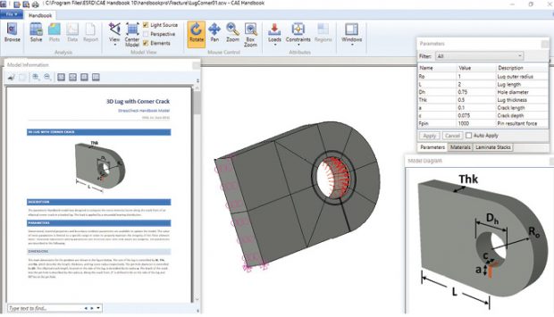 Fig. 1: CAE Handbook layout.
The Windows icon allows for the selection of visible windows. The windows can then be arranged by the user. On the left I am showing the Model Information window, which is a document describing the 3D Lug with Corner Crack Model. This can be printed or saved as a PDF. In the center is a plot of the FEA model, which will be analyzed, showing the mesh, loads and boundary conditions. On the upper right is the input dialog box for the lug and crack geometry, loading and materials. Below that is a diagram showing lug and crack geometry definitions.
I am using the default settings for this example. The lug is 2 in. wide and 2 in. long. The hole is concentric with the lug and has a diameter of 0.5 in. The crack is at 90° to the lug axis and is situated on the lower half of the lug. It is a quarter crack starting at the corner. The aspect ratio and size are controlled via crack length and depth inputs. Fig. 2 shows the starting crack and the prebuilt mesh provided to accommodate it.
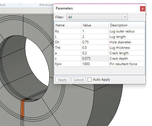 Fig. 2: Starting crack parameters and mesh.
The load is defined as a sine distributed bearing load along the lug axis. The magnitude is set by the user, 1000 lbf in my case. The cut face of the lug is constrained axially, but free to shrink by using an additional minimum constraint set.
There are an additional set of parameter-based rules, which prevent the user from inputting inadmissible geometry (negative volumes), crack shapes that are too shallow and lug configurations outside a reasonable range.
The FEA model is analyzed using the StressCheck solver from ESRD. This solver uses an automatic p-version method focused on solution convergence [1]. Each element can develop its own required order (p value) of internal shape function. A single element can handle very steep stress gradients. This contrasts with the more traditional h-element method, which requires an increasing number of elements to handle areas of steep stress gradient. The StressCheck solver allows automatic stress convergence to be achieved by running a series of analyses. The p value of the elements adapts until a target convergence criterion is met. The convergence history is plotted by default.
This approach ties in well with ESRD’s CAE Handbook methodology. The initial lug mesh has been defined by the FEA expert who built the model and compiled it into the CAE Handbook example. The model has been tested within the range of geometric variations defined by the geometry and associated rules. The starting mesh is structured to optimize the convergence performance. The recommended geometric grading of the mesh to deal with the singularity at the crack tip has also been predefined. Fig. 2 shows a very simple mesh schema, with few elements, but these represent well-defined domains within which to enhance the internal shape function. This avoids the need for the user to worry about controlling the mesh and provides consistency and reliability in the usage of the model.
The CAE Handbook is a form of templating. An expert FEA user can set up a model with one or more parts using Linear, Modal, Buckling or Nonlinear StressCheck solver solutions. In the case of the cracked lug, the Contour Integral Method is used to predict the required Stress Intensity Factors. The Model Information window, Parameters window and all the other input windows can be set up by the expert, following the guidelines in the CAE Handbook author’s guide. This is ideal for companies with repetitive analysis requirements. In my case, some 40 years ago I had to carry out exhaustive lug damage tolerance analyses checks on the Tornado combat aircraft. A tool like this would have meant turning that work around far more quickly and delegating much of the analyses.
With the model parameters set up, just click on the solve icon. A solution log shows the runtime history—eight analyses are used and the numbers of degrees of freedom (DOF) increase as the polynomial order is increased.
Once the analyses are complete—the convergence history is output in graphical form. ESRD places great emphasis on convergence checking and a variety of error measures can be chosen. I selected Total Potential Energy versus DOF. However, I could have chosen Convergence Rate or Percentage Error against DOF or Run Number.
The output that the user can see in the Handbook is controlled by its original author. In this case, an overview of the von Mises stress is part of the output available, as shown in Fig. 3.
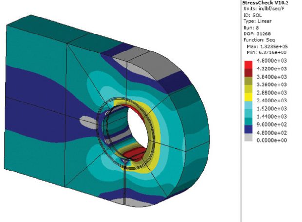 Fig. 3: Overview of von Mises stress.
However, in my case the Stress Intensity factors around the crack front are the most important result. From these values, the tendency for crack propagation can be estimated, together with the likely configuration of the crack development. By running a series of analyses and using the Paris Law, the crack propagation rate can also be estimated.
Convergence check plots on the Stress Intensity Factor at the two ends of the crack are also available. All the images, xy plots and data tables are available in a predefined report format, available for exporting as an xps file.
Note that the parent StressCheck solver has been used extensively in the aerospace industry for modeling fatigue cracking and delamination of a wide variety of fittings and joints [2]. The CAE Handbook examples are an interesting and easily accessible subset of that work.
The T Joint Structure
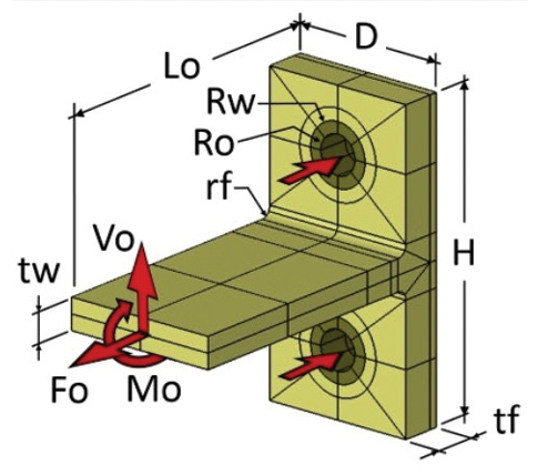 Fig. 4: T joint configuration and loading.
The T joint structure to be analyzed is shown in Fig. 4. The image is taken from the CEA Handbook Model Diagram. I was interested to compare the results of the StressCheck solutions against approximate hand calculation assumptions. The ESRD experts kindly helped me by modifying the T joint CAE Handbook model to prove additional contact pressure output.
The figure shows the main parameters to be input. In my case the only applied loading is a vertical tensile load. I used the default values for the handbook example, which provide for a 6-in.-wide bracket, 3 in. deep and 6 in. high. Flange thickness is 0.8 in. and vertical web thickness is 0.6 in. The fillet radius is 0.2 in. A 0.375 radius bolt is used, with a 0.6-in. radius washer face. A flexible backing structure is assumed, with a stiffness proportional to the flange in the normal direction. Bolt shank and washer axial stiffness are set to the same stiffness value.
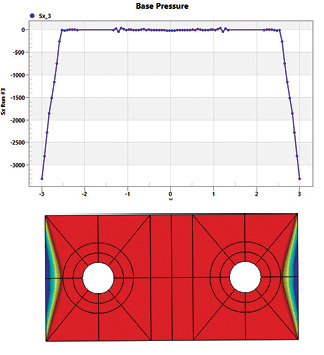 Fig. 5: Contact stress distribution with no preload, upper and centerline stress, lower.
There is an option to apply a bolt preload via bolt elongation, but initially I wanted to check the basic bolt prying action without a bolt preload. I used 10,000 lbf applied vertically. Fig. 5, lower, shows the “prying” normal contact stress outboard of the bolt washer faces. The red contour is at zero stress. It is interesting that the variation across the depth of the flange falls to zero at the front and back edges. The distribution is assumed constant in the simple hand calculations. The graph in Fig. 5, upper, shows the centerline contact stress. The distribution agrees well with the triangular distribution often assumed in hand calculations.
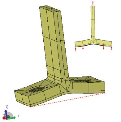 Fig. 6: Bolt reaction system (inset) and deformed shape plot.
The “prying” action is highlighted by the deformed shape plot, shown in Fig. 6. The end edges of the flange form the “prying” points with corresponding reactions, creating higher bolt loads than if the flange was infinitely stiff.
There are many semi-empirical methods for calculating prying force. If the prying force distribution is assumed to act at the flange edge, one classical solution is:
Q = bF/(2a)
Q is the prying force, 2F is total applied load, a is distance from edge to line of bolt reaction, b is distance from the web face to the line of bolt reaction.
Using this hand calculation, the bolt force is 6,653 lbf per bolt (prying reaction is 1,653 lbf).
Reference [3] includes the flange thickness in the calculation. I changed the effective distances a and b using reference 4. The calculation then becomes:
Q = F(3b’/8a’-t^3/20)
Where t is the flange thickness and a’ = a+r , b’=b-r, where r is the bolt radius.
The bolt force is now 6,112 lbf and the prying reaction is 1,112 lbf.
The CAE Handbook result is 6,059 lbf bolt force and 1,059 prying reaction and represents a more sophisticated solution.
I have also plotted the maximum principal stress as shown in Fig. 7. The peak value is 24,540 psi.
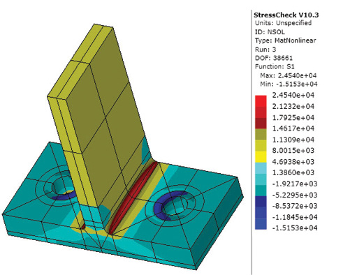 Fig. 7: Maximum principal stress for baseline model.
Factors such as flange nonlinear contact and hence stiffness have historically made hand calculation difficult. I have not validated the current FEA results against test, but have used this configuration as a baseline to investigate bolt load with applied load, under constant preload. The CAE Handbook is ideal for this type of study, providing fast turnaround.
The bolt elongation due to preload is now set at 0.004 in. The bolt preload is checked by running an analysis without applied load. The preload developed is 53,042 lbf per bolt. The distribution of normal stress under contact is in Fig. 8.
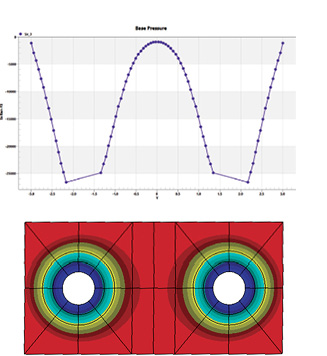 Fig. 8: Centerline plot (upper) and contour plot (lower) of contact stress under preload only.
The distribution is virtually concentric around each bolt. The stress falls off in a linear profile, apart from under the T joint web region.
With fully applied load of 130,000 lbf the stress distribution is very different, as shown in Fig. 9.
In classical bolt joint calculations, when a critical load is reached, the flange is assumed to separate from the backing plate to which it is clamped. This is described as preload “breakout.” Fig. 9 shows that there is still contact at a high total applied load level of 130,000 lbf, with a prying type action developed at the flange edges. The flange and backing plate are flexible in this FEA study. In classical bolt joint calculations, they are assumed to be rigid, allowing a well-defined breakout point.
The variation of bolt load with applied load per bolt can be shown to see the expected preloaded bolt breakout trend, with the preload having a near constant value up to the breakout applied load and then increasing linearly with applied load. The breakout is not an abrupt transition, as in classical calculations, but by around 35,000 lbf applied load the transition is complete.
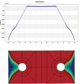 Fig. 9: Centerline plot (upper) and contour plot (lower) of contact stress under full load.
In conclusion, the examples I used from the ESRD CAE Handbook library allowed me to investigate two different scenarios quickly. In the T-joint case, a useful extension beyond classical methods is found. Because I did not have to focus on FEA model setup, I could concentrate on planning the studies and interpreting the results. All models and documentation are loaded into the library, so it was easy to pick up the thread when I revisited the studies after a long break.
I look forward to trying the next stage, building up my own CAE Handbook example using StressCheck.
References
- Szabo B and Babuska I. Introduction to Finite Element Analysis. Formulation, Verification and Validation. John Wiley & Sons Ltd., Chichester, UK, 2011.
- Szabo B and Babuska I. Computation of the amplitude of stress singular terms for cracks and reentrant corners. Fracture Mechanics: Nineteenth Symposium ASTM STP 969. T. A. Cruse, Ed., American Society for Testing and Materials, Philadelphia (1988) 101–124.
- Douty RT and McGuire W. “High Strength Bolted Moment Connections,” Journal of the Structural Division, Vol. ST2, 1965, pp. 101–128.
- Struik JHA and De Back J. Tests on bolted T-stubs with respect to a bolted beam-to-column connection,” Stevin Laboratory report 6-69-13, Delft University of Technology, The Netherlands, 1969.
Subscribe to our FREE magazine, FREE email newsletters or both!
Latest News
About the Author
Tony Abbey is a consultant analyst with his own company, FETraining. He also works as training manager for NAFEMS, responsible for developing and implementing training classes, including e-learning classes. Send e-mail about this article to [email protected].
Follow DE