Visualization of the noise pressure level outside the gearbox and vibration-induced von Mises stress in its housing. Image made using COMSOL Multiphysics software; courtesy of COMSOL.

Latest News
August 1, 2018
At first glance, the COMSOL Multiphysics user interface, as shown in Fig. 1, looks similar to many other finite element analysis (FEA) based products. The top ribbon contains a series of tabs that give access to Geometry, Materials, Mesh, Study and Results. This suggests a familiar workflow through the pre-processing, solution and post-processing stages of analysis.
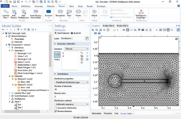
Fig. 1: COMSOL user interface. Images courtesy of Tony Abbey.
However, there is a set of other tab names that give a hint of the much wider applicability of COMSOL Multiphysics. These include Definitions, Physics and Developer.
Core COMSOL Multiphysics has Solid Mechanics as the single physics interface. However, add-on Physics Modules include:
- Electromagnetics
- Structural Mechanics and Acoustics
- Fluid Flow and Heat Transfer
- Chemical Engineering
Building a Structural Model
The first task in this review is to build a simple 2D model. The model details are shown schematically in the Model Builder window, as shown in Fig. 2. These will be referenced during the model build.
Each major subset of the model tree in the Model Builder window is called a node. The primary nodes shown are Global Definitions, Component, Study and Results. Sub nodes can be seen, under Component for example, controlling Geometry, Materials, Solid Mechanics and the Mesh.
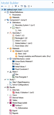
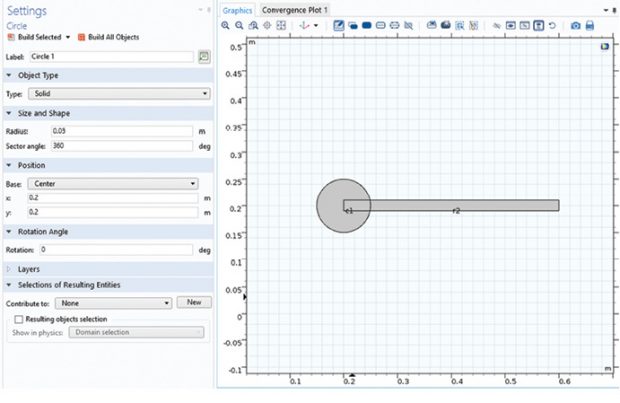
Fig. 3 shows the single component created for a Normal Modes analysis. The model is a very simple 2D shape, constructed from the union of a circle and a rectangle. Fig. 3 also shows the graphics window with the geometry and a typical Settings form, in this case for the circle definition. The Circle, Rectangle and Union objects are shown under the Geometry node in Fig. 2. The Delete Entities object trims the redundant interior boundaries of the combined shape. Finally, the Form Union object creates the shape.
A full CAD import and manipulation capability is present within COMSOL Multiphysics, so much more sophisticated geometry can be handled.
The material is applied next, and definitions appear under the Materials node. Note that the shape has two domains—the original circle and the rectangle. The material is applied to both.
Under the Solid Mechanics node, the material is defined as linear elastic, using plane strain assumptions. All the boundaries around the periphery of the combined shape are defined as free, all initial displacements are set as zero and then a fixed constraint is applied to the circle domain. The order of the objects under each node is important as it dictates the build logic. In this case, the constrained circle overrides the free boundary at the circle edges.
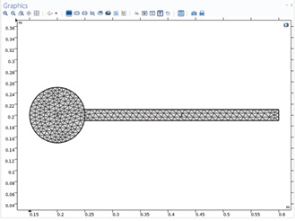
The mesh controls under the Mesh node allow for a size control over both domains. The mesh can be automatically calibrated for different physics—Structural Analysis in this case, or optionally Fluid Dynamics, Plasma Flow or whatever other types of physics are appropriate. I have chosen the Free Triangular mesh format. Additional meshing controls are available.
I have overridden the defaults and produced a mesh as shown in Fig. 4.
I have selected an Eigenfrequency (Normal Modes) analysis as the study type.
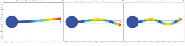
The Compute icon in the study tab launches the analysis. Fig. 5 shows the first three mode shapes. The frequencies are 5.88, 36.21 and 98.7 Hz, respectively.
Moving to a Coupled CFD and Structural Analysis
Having established the baseline frequencies for the structural shape, I moved on to a coupled fluid-structure interaction (FSI) analysis. The shape defined is a classic benchmark and I have borrowed from the COMSOL verification example that uses the results of an independent analysis.1
The circular body under a low speed steady fluid flow sheds a series of alternating vortices known as a von Kármán street. This creates an interaction between the trailing plate and the vortex dominated fluid flow. The verification example uses a fluid similar to gelatin and a flexible rubber-like solid material. I have stiffened the solid material to reduce the amplitude of oscillation, but kept all the other parameters the same. The stiffened material was also used in the normal modes analysis.
The study is reset to be time dependent using Solid Mechanics (structural response), Laminar Flow (fluid response), a moving mesh and a fully coupled FSI. The time step and duration are also set.
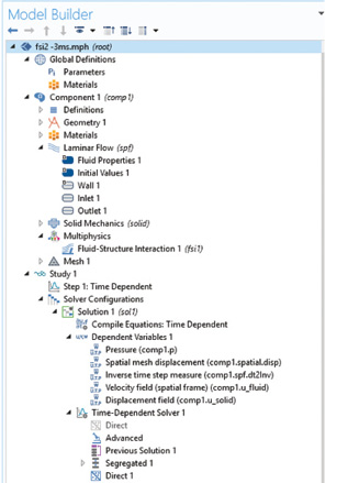
The revised model tree is shown in Fig. 6. The dependent variables are set as the displacements, velocity and pressure. There are also a set of Laminar Flow and FSI solution settings seen in Fig. 6, which I have used, based directly on the COMSOL application example.
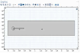
The geometry is adjusted by introducing a rectangle to represent a channel through which the fluid flows (Fig. 7). A split line (not shown) is placed aft of the training edge to control the fluid mesh.
The Solid Mechanics module is modified slightly by adding a small vertical force at the trailing edge to promote a level of eccentricity to aid formation of the von Kármán vortices.
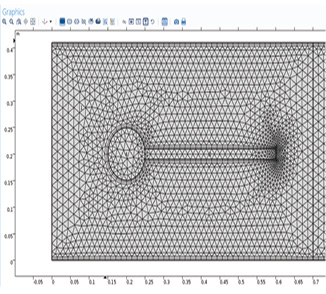
The mesh settings are modified to control the mesh in the fluid domain. The fluid mesh around the structural shape is shown in Fig. 8.
The fluid material is added and allocated to the fluid domain.
Within the Laminar Flow node, properties are set to be incompressible with no turbulence. Within the Wall node, the fluid boundaries in contact with the channel wall are defined as no slip.
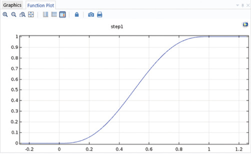
The initial flow speed is set to zero and then rises over a 1-second time period. The function to define the transition allows for an abrupt step or a user-controlled smoothing function. The latter was defined as shown in Fig. 9.
The initial flow is also given a short “kick” to help promote flow instability at 1.5 seconds. This is done via another function, this time defined as the Gaussian pulse shown in Fig. 10.
The flow at the inlet is scaled through time as shown, but is spatially defined as a parabolic distribution, typical of a fully developed flow in a channel section. An expression with mean flow velocity and channel height is input into the Inlet definition in the Laminar Flow node. The Outlet is defined with zero backpressure.
The Multiphysics node controls the FSI coupling—and is defined between the Laminar Flow physics and Solid Mechanics physics.
Two Global Variable Probe definitions are set up. One integrates the “x” component of pressure over the structural bounding surface to calculate the total drag. The second integrates the “y” component to calculate the total lift. Lift and drag are then available as a function of time.
A Domain Point Probe is defined at the trailing edge and horizontal and vertical displacement components assigned to it. They are available as a function of time.
Results
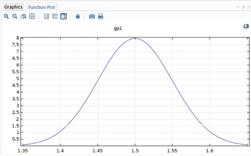
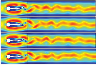
Fig. 11 shows snapshots of the fluid velocity captured between 4 and 6 seconds of the event.
The von Kármán vortex street can be clearly seen. The oscillating nature of the opposing vortices induces motion in the plate, which in turn effects the fluid flow. The series of 101 plot states created during the analysis can be animated, with control over frame rate allowing good visualization of the vortices to be achieved.
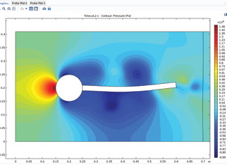
A snapshot of pressure distribution is shown in Fig. 12. The pressure was also animated through time. The local intensity of pressure is moving up and down the plate length, as well as oscillating from top surface to bottom surface. The second bending mode of the plate is playing an important role in the interaction.
The frequency of oscillation can be quantified using the trailing edge displacement probes set up earlier. The vertical oscillation is shown in Fig. 13.
The lower time history plot in Fig. 13 shows a steady state oscillation at 2 m/s flow rate over the time of 4 to 5 seconds. The frequency of this oscillation is 5.5 Hz, which agrees closely with the benchmark.1 The theoretical vortex shedding frequency with the sphere in isolation is 3.57 Hz, which gives an indication of the level of interaction introduced by the plate.
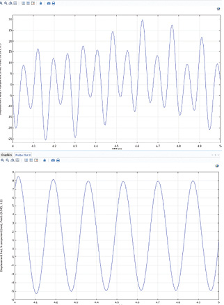
The upper time history plot shows a more complex oscillation achieved with a higher flow speed of 3 m/s. I used a Fourier analysis tool available within COMSOL Multiphysics to operate on this output signal. The frequency content is now split between 7.4 Hz and 14.1 Hz.
The total lift and drag are also available as time history plots.
An application reported by COMSOL2 demonstrates how another layer of physics could be added to the coupled FSI scenario. Nokia is investigating cantilever plate-like fans driven by a piezoelectric sandwich mounted on the plate. They used COMSOL to predict fluid flow generated from the fans, hence incorporating mechanical, fluid and piezoelectric physics.
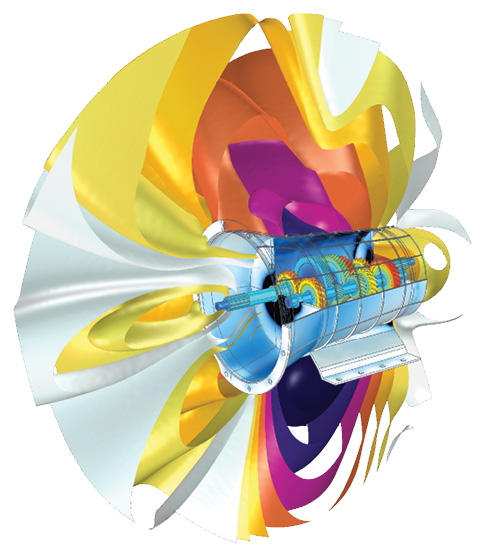
Fig. 14: Visualization of the noise pressure level outside the gearbox and vibration-induced von Mises stress in its housing. Image made using COMSOL Multiphysics software; courtesy of COMSOL.
I have kept to a very simple 2D simulation, based on time constraints. However, the scope of COMSOL in CFD and FSI application extends well beyond this, as the examples in Figs. 14 and 15 show.
Application Builder
I set up a Global Parameter for the flow speed. This enabled simple control of the series of analyses, with a range of flow speeds between 2 m/s and 3 m/s. The COMSOL Application Builder is perfect for further exploration. This is available in any COMSOL simulation and automatically builds input parameters and result quantities from the simulation into one or more forms. The forms then become the basis for a stand-alone application, which will reproduce the simulation. A set of layout configuration tools and programming support allow for documentation and customization of the application.
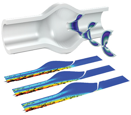
Fig. 15: Visualization of deformation, von Mises stress and velocity magnitude in an FSI analysis, including contact modeling, of a heart valve. Image made using COMSOL Multiphysics software and courtesy of COMSOL.
Considering the breadth of physics that COMSOL brings to simulation, this is a significant tool. It allows a collaborative application developed by a group of specialists in different fields of physics to be deployed to other users within a company. Checks and balances can be incorporated to ensure less experienced users can produce meaningful results. A complete library of pre-built applications is available within COMSOL Multiphysics.
Conclusion
This overview really just scratches the surface of the capabilities within COMSOL. It is clear that if you have the scientific or engineering knowledge to dive deeply into any of the areas of physics provided, then you will be able to create innovative simulations to many applications. My work on this review did show me how limited my range of knowledge is! However, I did find the COMSOL documentation, examples and references extremely helpful in my efforts to brush off some cobwebs and stretch my knowledge further.
References
1. Proposal for numerical benchmarking of fluid-structure interaction between an elastic object and laminar incompressible flow. Stefan Turek and Jaroslav Hron, Institute for Applied Mathematics and Numerics, University of Dortmund, Vogelpothsweg 87, 44227 Dortmund, Germany.
2. It’s a bird, it’s a plane: Flow patterns around an oscillating piezoelectric fan blade. Sarah Fields. COMSOL magazine October 2017.
Tony Abbey partners with NAFEMS, and is responsible for developing and implementing training classes, including a wide range of e-Learning classes. Check out the range of courses available: nafems.org/e-learning or contact [email protected] for details.
More COMSOL Coverage
Subscribe to our FREE magazine, FREE email newsletters or both!
Latest News
About the Author
Tony Abbey is a consultant analyst with his own company, FETraining. He also works as training manager for NAFEMS, responsible for developing and implementing training classes, including e-learning classes. Send e-mail about this article to [email protected].
Follow DE