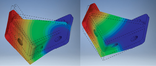
The first two modes: Mode 1 (left) 1044 Hz, Mode 2 (right) 1221 Hz.

Latest News
September 1, 2018
A few years ago, Autodesk acquired NEi Software, a small company that developed an independent finite element analysis (FEA) solver that closely emulated the traditional Nastran input and output structure. Since then, Autodesk has embedded much of the solver technology into its Autodesk Inventor environment as Autodesk Nastran In-CAD. The full solver capability also continues to be available as a standalone product, Autodesk Nastran.
For this review I have created a simple bracket model. The file is available for download at autodesknastran. Versions using Parasolid, Autodesk Inventor and SOLIDWORKS formats are available. The Autodesk Nastran input files and result files are also available for download.
User Interface
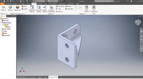
Fig. 1 shows the Autodesk Inventor user interface (UI), with the bracket geometry shown. The layout is traditional, with a tree view, graphics area and a main menu running horizontally across the top. Autodesk refers to this as the ribbon. Selecting a tab on the ribbon opens a set of commands and drop-down menus. Fig. 1 shows the Tools options selected.
I opened the Parasolid version of the geometry and was interested to see how the geometry conversion was handled. The source file holds the default input units, which in this case picks up meter units. This can be changed to inches easily. However, it is always a good idea to check units and dimensions during an import. The Inspect tab has an easy-to-use measure tool, which is always a good check. The vertical bracket edge is correctly reported as 2.75 in.
Users can check model units by using Document Settings under the Tools tab. The units are reported as inches and pound mass. I was a bit skeptical as to whether strict mass units were being used. I was carrying out a dynamic analysis, so it is important to be clear on this point.
I selected alloy steel from the provided material list. It is also straightforward to set up a new material library or define a new material. The file created is clearly indicated and can be copied or made centrally accessible.
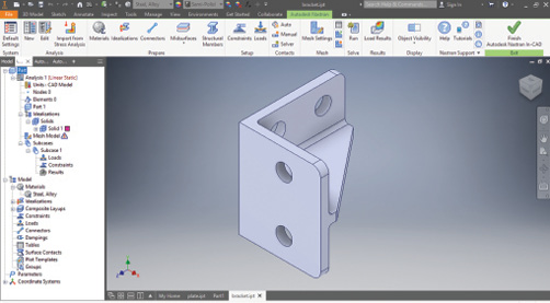
Right mouse-clicking on the Solid1 object in the part tree view allows the body properties to be listed. The results are a ‘mass’ of 1.279 units and a volume of 4.578 cubic in. This confirms that the Autodesk material is using a weight density and that this is the weight of the part. The simulation tool is selected by using the Environments tab and then the Autodesk Nastran In-CAD icon. A new ribbon and tree view appears as shown in Fig. 2.
Tabs appear that cover the usual FEA actions of pre-processing, analysis control and post-processing. The new tree view is in two sections: the Analysis tree that shows the options applied to the current part for this analysis and the model tree that shows all the options that can be set. The options defined in the model tree are available for use in the Analysis but are not activated until dragged across or created directly from within the Analysis tree.
The solid geometry present has spawned a 3D solid “Idealization” object, as shown in Fig. 2, with inherited part material properties. There are two other Idealization options that can be associated with the model using 2D shell elements or 1D beam elements. The 2D shell option requires surfaces to be designated for meshing. There are three possible approaches: automatic creation of Thin Bodies, Mid-surfacing and Offset Surfaces. Thin Body creation uses a criterion of 20:1 for length to thickness. The bracket is too “chunky” to pass this test and so no automatic surfaces can be created. Mid-surfacing attempts to create mid-surfaces through the solid body. Offset surfacing allows external body surfaces to be copied to an interior position via an offset. Experimenting with both methods resulted in a gap between the bracket faces and the central gusset. A more general approach would be to create the required surfaces directly in Autodesk Inventor. 1D beam elements can be meshed from Autodesk Inventor Frame Members.
Meshing
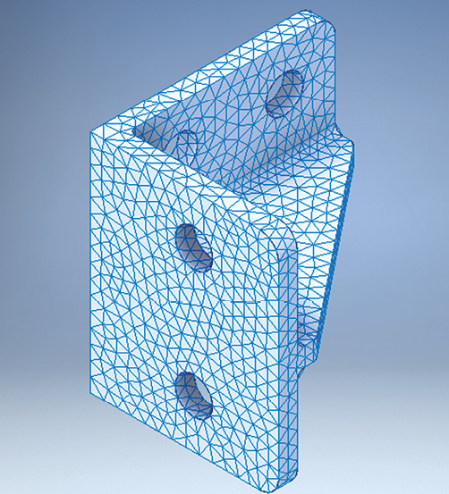
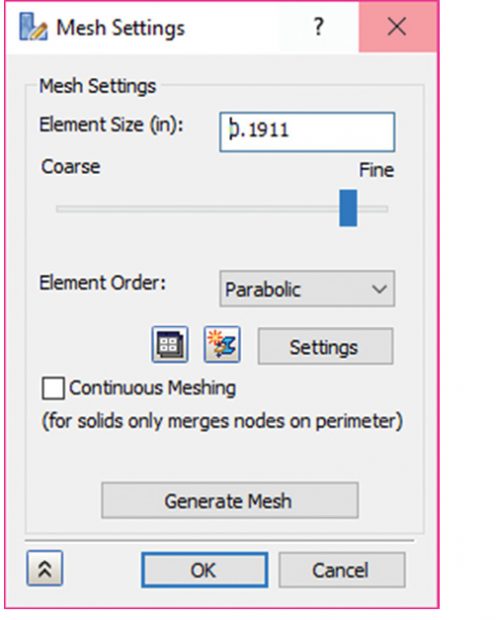
Fig. 2 shows a warning that a mesh is required. Right-clicking on Mesh Model or using the ribbon icon generates the mesh. The result is shown in Fig. 3. Right-clicking on the Model Mesh or using the ribbon icon accesses the mesh settings shown in Fig. 4.
The default or global mesh size is 0.1911 in. This is a very useful parameter, as it indicates the starting point for adding local refinement. Guessing a value can result in a huge number of elements or a very coarse mesh. Reducing the global size is one refinement option, but it is a very expensive solution. The number of elements with the default size is 8,332.
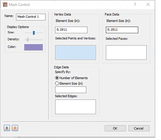
Halving the element size to 0.095 gives 67,844 elements, halving again to 0.0475 gives 474,797 elements. As usual the objective is to put fine mesh control where it matters. Autodesk Nastran has local mesh controls as shown in Fig. 5.

Any number of local controls can be used to target vertex, line or surface geometry. As an exercise, I assumed that a fine mesh is needed around the bolt holes on the horizontal faces to investigate stresses. Fig. 6 shows the result of increasing the mesh refinement locally on the edges of both of these holes.
The element relative local size and element count is:
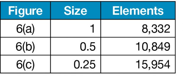
The final Fig. 6(d) is a result of reducing the Element Growth Rate to 1.2 from a default of 1.6. The effect is to keep a fine mesh bias over a larger distance away from the bolt hole. The number of elements using this method is 33,113.
Analysis Setup
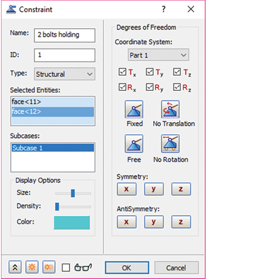
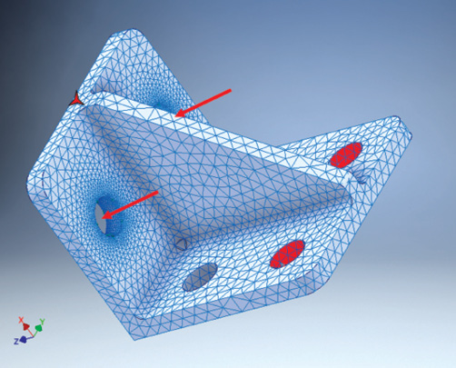
The bracket is assumed to be connected to a stiff backing structure at the outer pair of bolt holes on the YZ plane flange. This represents a case where the inner bolt pair has been missed in assembly. The bolts act as a standoff, rather than clamping the structure to the backing. The constraint setup is shown in Fig. 7.
The constrained degrees of freedom (DOF) can be set manually, or simple constraint options such as symmetry can be invoked. Cylindrical constraints such as bolt hole rotation can be set up, but the required coordinate system must be defined in the Autodesk Inventor Model first and then referenced here.
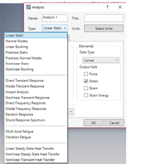
The task for this overview is to carry out a Normal Modes analysis and a subsequent Modal Transient Dynamic analysis on the bracket. The default analysis is linear static. Right mouse-clicking on the Analysis object in the Analysis tree, and selecting edit allows any analysis to be set up, as shown in Fig. 8.
At the time of this writing, all analysis options are available with a standard license. The Autodesk Nastran standalone solver is also bundled with no restrictions on the input file origin.
Selecting Normal Modes allows control over output. I deselected reaction forces and stress—only the eigenvectors (displacements) have any meaning. An additional control object named Modal Setup 1 is created in the Analysis tree and gives access to further context-based parameters. I kept all defaults, which included the number of modes and extraction method, but opted to save the modal database.
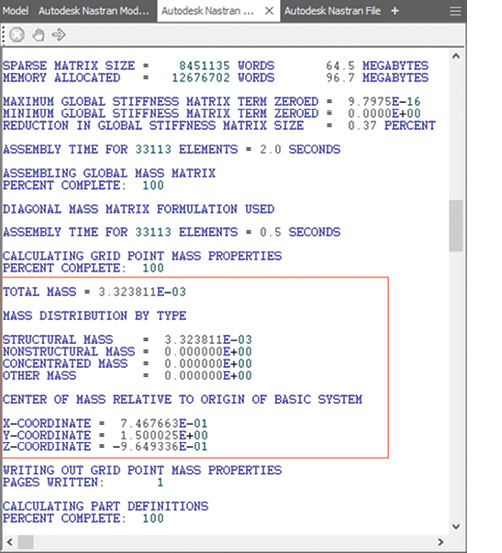
Running the analysis creates two more view panels alongside the Model (Autodesk Inventor) and Autodesk Nastran Model Tree. These are shown in Fig. 9.
The Nastran output file tab has been selected in Fig. 9. I have highlighted the mass property calculations in the Nastran solver. The structural mass is reported as 3.3238e-3 units. This is the correct value in pounds mass (lbm). This is checked by dividing the weight by gravity, 386.4 inches per second squared. The translator between Autodesk Inventor and Autodesk Nastran appears to be hardwired to make this weight-to-mass conversion; it’s something to consider.
The output file is useful for debugging and understanding the calculation flow. Experienced analysts will welcome this additional insight, and it is a great tool for newcomers to start to investigate the process more deeply.
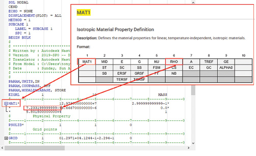
In that vein, the other new tab created is the Autodesk Nastran input file, shown in Fig. 10.
The syntax of the input file takes some effort to interpret, but will give a deeper understanding of the analysis. I have overlaid part of the material property (MAT1) description from the documentation. The Nastran documentation can be loaded locally; the default is online. Hitting F1 while highlighting the input file will spawn the documentation. A search will then take users to the relevant data. The NEi Nastran original version was fully context sensitive and the relevant documentation was spawned automatically. I hope Autodesk Nastran’s developers can reincorporate this to enhance the learning curve and productivity.
In Fig. 10 I have highlighted the density term RHO. The Nastran input file is definitive and hence it is useful to be able to check the translation within the Model database.
Analysis Results
The first two modes from the analysis results are shown in Fig. 11. The plots show the first bending mode and the first torsional mode. I have modified the default settings to give a banded contour view, switched element edges off and deselected maximum and minimum markers. It is straightforward to move between the frequencies, retaining this view. Animation also has good controls. I increased the number of frames to 24 and used the oscillate option. I found it easier to move between modes with animation by using the control panel available from the Analysis tree view, rather than the ribbon controls.
Running a Normal Modes analysis also spawns a set of XY plots. The first is a Frequency versus Mode Number plot, and the next six are Modal Effective mass plots: one for each DOF.
These plots are important for carrying out a modal survey. In this case, the first two modes are similar at relatively low frequencies, but the frequencies climb rapidly with more complex modes. A typical response spectrum cutoff may be at 2000 Hz, and the first two modes are the only two of concern. Alternatively, if a payload is attached to the bracket, approximate hand calculations can estimate the drop in frequency and whether higher modes may become important. The modal effective mass graph shows mode 1 contributing in a vertical (Z) sense, but mode 2 does not. This allows excellent predictions for base motion excitation and approximate indications for external excitation.
For the next task, I created a transient analysis with a vertical (Z) impulse being applied at the two bolts in the XY plane. The setup is shown in Fig. 12.
I edited the Normal Modes analysis and converted it to a Modal Transient analysis. This spawned new objects in the tree view. There are other possibilities, such as creating a duplicate analysis and then editing. The motivation is to inherit the Normal Modes analysis settings.
I edited the Modal Setup object to reuse the Modal database created in the Normal Modes analysis. For a large model this can be a significant saving in resource and run time. Damping is defined via the Damping object in the tree view. Constant Modal damping is very easy to apply— just defining the value. I used 1% critical damping. Rayleigh, Structural and variable Modal damping are all available.
Using the Loads object in the tree view, loading is applied in the usual way as a static loading, with an option to create the time dependency on the fly via a table. Alternatively, a table can be separately defined, with the ability to paste external data.
Time step size and number of time steps are input via the Dynamics Setup object created in the tree view. If you know the step size and duration, which is the typical case, the number of steps is calculated automatically.
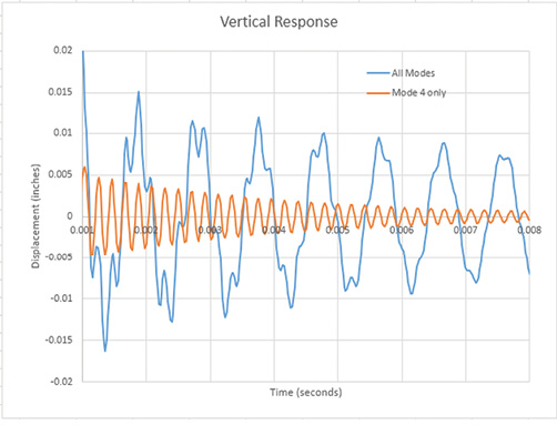
The analysis results are presented as a vertical (Z) deflection time history at the edge node indicated by the red star in Fig. 12. Results are shown in Fig. 13 for two analysis runs.
The first analysis used the standard Nastran file setup from Autodesk In-CAD. The second analysis used a modified Nastran file to look at the contribution from mode 4 only. The file modification was carried out from within the Autodesk Nastran File tab using the direct editing tools available and the local help documentation.
The ability to filter modes to gain understanding in this way is very powerful. The same modal database is reused each time.
FEA-CAD Combo
Autodesk Nastran In-CAD is an interesting combination of a traditional FEA tool embedded in a CAD environment. Much of the product’s richness is apparent in the embedded solution. Together with the availability of the full standalone product, this will be attractive to experienced analysts. On the other hand, the user-friendly CAD-like environment is attractive to beginners or infrequent users of FEA. The availability of all analysis types at a single licensing level is good news for all.
More Autodesk Coverage
Subscribe to our FREE magazine, FREE email newsletters or both!
Latest News
About the Author
Tony Abbey is a consultant analyst with his own company, FETraining. He also works as training manager for NAFEMS, responsible for developing and implementing training classes, including e-learning classes. Send e-mail about this article to [email protected].
Follow DE