Latest News
April 1, 2014
By Richard Gustavson
Would you like to assure that your single or multiple product system designs always satisfy technological needs and company economic requirements? Now you can do both during all stages of the product/system design process.
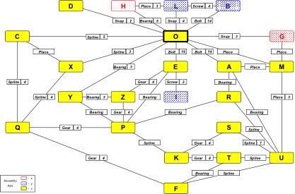 Figure 1: Logic Schematic for an Assembly Process.
Individual Tasks and Mating Requirements are shown.
Assembly Sequence is
O, C, X, D, H, M, A, U, G, R, S, K, T, F, Q, Y, P, Z, E, I, B, L
Methods for determining the optimum combination of applicable resource-types that can perform a specified set of tasks have generally been a mixture of sometimes clever procedures for a few of the phases of the overall system design process. Most of the time, technical requirements are investigated independently of cost considerations. Such a process usually becomes iterative quickly, and wastes time and money. Today, rigorous methods are available for combining economics and technology such that both are simultaneously optimized. The procedures to be described are not a computerized trial-and-error scheme; they utilize the enlightened techniques of synthesis (solutions always satisfy the requirements — in this case, two normally disparate activities are combined). These methods were developed over more than 25 years utilizing a wide variety (in size, complexity and production quantity) of actual products.
Requirements for What is to be Accomplished
Whether the process is design, fabrication or assembly, a collection of tasks must be accomplished. Various resource-types (manual, fixed automation, programmable automation) may be utilized. Since there are typically many more applicable resource-types, assembly will be used in the examples for this article. Figure 1 exhibits a logic schematic for the tasks and inter-relationships of a moderately complex assembly process.
A Task/Resource Matrix
For any set of tasks to be accomplished, two major activities must be performed:
1. Establish the task sequence — automated methods exist for many sub-types of assembly (e.g. see caption for Figure 1).
2. Select an appropriate group of applicable resource-types — each has cost and performance characteristics.
When properly combined, these two procedures can generate a task/resource matrix that exhibits the cost and performance characteristics for the specified alternatives. The goal is to establish the combination of resource-types that satisfies the throughput requirements at the lowest cost. For manufacturing systems, production volume (using year, quarter, month, week, day, hour, minute or unit) and corporate economic requirements (e.g. minimum attractive rate-of-return, maximum investment, and planning horizon) are the primary conditions.
[gallery columns=“2” link=“file” ids=”/article/wp-content/uploads/2014/04/Figure2.jpg|Figure 2 General Solution
Rating is a function of Unit Cost, Total Investment, & Station Count
The Optimum is not at Maximum Available Time, /article/wp-content/uploads/2014/04/Figure3.jpg|Figure 3 Specific Solution One of the Possible Loop System Layouts for the Best System Black dot defines bottleneck station Yellow dot defines maximum effort station”]
General Solutions
Line balancing has often been the basic criterion for finding the best assembly system. Unfortunately this procedure only applies to a mostly manual process at, or near, the maximum available shift time. It will be a by-product of this innovative method since solutions over a wide throughput range are provided. The optimum system is determined using a rating that requires a proportional weighting for three “floating” parameters: unit cost, total investment, and number of workstations. A general solution example is shown as a column chart in Figure 2. Note that the optimum solution does not occur at the maximum available time. Such a result generally occurs when few, if any, manual stations are part of the system.
Specific Solution
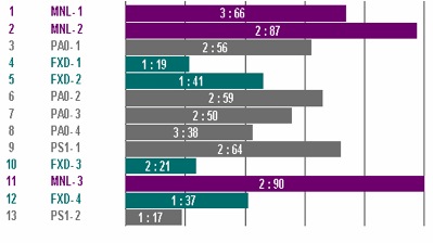 Figure 4: Comparison of Effort Required at each Workstation
Can be used to assign personnel in capability order
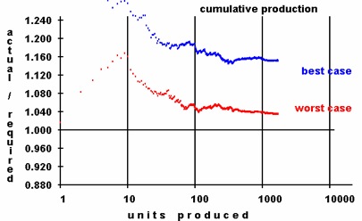 Figure 5: Stochastic Behavior of a System using Triangular Distributions. Sometimes, the worst case time ratio is less than 1.0. This could also be true for the best case ratio.
Picking the highest rated solution from results such as shown in Figure 2 (or any other Portion of Total Available Time) permits eventual display of a simplified bounding box geometric layout (Figure 3). When the degree-of-difficulty for each task is imposed, a bar chart for the expected total difficulty at each workstation can be presented (Figure 4); this information readily permits optimum assignment of direct labor when required.
Variable Workstation Time
Although these system design procedures are primarily deterministic, stochastic information for discrete (as opposed to continuous) manufacturing systems are also provided. Best case conditions occur when the same random number seed (r.n.s.) is used for all stations (a common assumption in simulation analyses), while worst case arises from using a different r.n.s. value for each workstation. The expected output divided by the nominal bottleneck output for an example system using triangular distributions can be seen in Figure 5. Exponential distributions have also been implemented; since longer times will be possible, they generally have lower throughput ratios than those shown.
A Spectrum of Solutions
When the number of times the total process is repeated during a prescribed time period (i.e. the production rate) is investigated over a wide range, different “best” systems will result. Figure 6 displays the typical relationship between two of the three factors that influence the RATING for a specific maximum shifts. The required number of each resource-type increases non-linearly as production requirements increase (Figure 7); this data provides the third RATING factor.
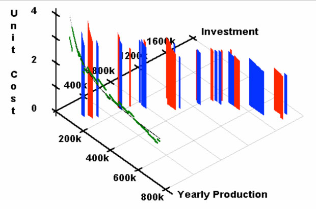 Figure 6: Solution Spectrum for a Single Product Relationship between production, investment and unit cost for a group of optimum systems.
Establishing the Most-Desirable System
Unit cost vs. yearly production behavior as seen in Figure 6 can be readily compared to similar results for a different number of shifts. Figure 8 exhibits the fact that every production volume will have an optimum shift condition. As an example, check the performance, cost and station count for 315000 units per year of the example assembly system.
Shifts | Utilization | Investment | Unit Cost | MNL | PS1 | PA0 | FXD |
1 | 0.937 | 1562k | 2.608 | 3 | 0 | 9 | 11 |
2 | 0.865 | 1017k | 2.494 | 3 | 2 | 4 | 4 |
3 | 0.987 | 519k | 2.140 | 3 | 0 | 3 | 1 |
[gallery columns=“2” link=“file” ids=”/article/wp-content/uploads/2014/04/Figure7.jpg|Figure 7: Solution Spectrum for a Single Product Number of each resource-type required for each optimum system,/article/wp-content/uploads/2014/04/Figure8.jpg|Figure 8: Establishing the Most Desirable System Unit Cost comparison for 1 shift, 2 shifts, and 3 shifts
Other comparisons (e.g. RATING) establish the same best case.”]
Combining Processes Using a Single System
Some manufacturers have established an assembly system that can produce a significant number of variations of a base product (e.g. panel meters); that is not the situation being discussed here. One of the ultimate goals of assembly systems is to have disparate products output by one arrangement of resource-types instead of each product requiring an independent system. Such a condition is only possible if the size, weight, and number of tasks required are somewhat similar for each product. The proverbial production lot size of one could then be possible.
Two Product Systems
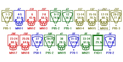 Figure 9(a): Best System Schematic for
Product 1 of a Two Product System. Each workstation shows: resource-type used, task(s) assigned, cycle time, and effort. Color denotes maximum degree-of-difficulty.
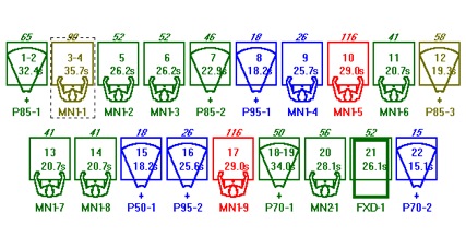 Figure 9(b): Best System Schematic for Product 2 of a Two Product System
To determine whether systems exist that can assemble two somewhat similar products over a wide range of production ratio, an expansion of the single product procedure has been implemented. An example, shown in Figure 9, presents the system schematic layout for two moderately different products; this result is from the synthesis procedure. Note the varying number of tasks, processing time, and difficulty using the same resource-type at each workstation. The maximum degree-of-difficulty for any task at a workstation is color coded according to:
Blue — straightforward task
Green — some difficulty likely
Yellow — hard to do; fixed automation may be possible
Red — arduous; must be done manually
When a range of production ratios for the two products is investigated, a number of systems can be determined that requires an exact same set of resource-types for a usually limited range of total yearly output for the two products. While Figure 10 exhibits discrete values, the maximum output for each system (identified by the required investment in thousands) is represented by a curve that extends beyond the leftmost and rightmost data points. Production ratio areas for combined systems being best or individual systems most desirable are readily identified.
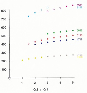 Figure 10: Example Two Product System Behavior showing that a number of systems are usable over typical ranges of maximum total yearly production. Solid circles for combined system’s best. Hollow circles for individual system’s best.
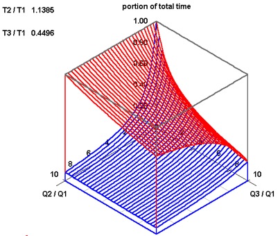 Figure 11: Three Product System Time Availability
for prescribed total time ratios and a range of production ratios.
Three Product Systems
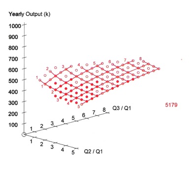 Figure 12: Three Product System Behavior
For this product grouping, less than 10 usable systems for the maximum production range of 200k to 1M are available. Solid circles for combined system best. Hollow circles for individual system best.
Adding a third reasonably similar product normally results in few widely usable systems. When both Q2/Q1 and Q3/Q1 production ratios (utilizing expected total processing time ratios T2/T1 and T3/T1) are evaluated over expected ranges, Figure 11 exhibits the portion of total time that will be specified as available for each of the three products. An x-y-z surface will be required to display maximum total production vs. production ratios; one example three product system is shown in Figure 12. An irregular area boundary curve will separate the best combined systems from the best individual systems.
Systems for More Than Three Unique Products
While more than three somewhat similar products might be produced using a single system, a very small number of usable examples have been found. No graphical representation is possible although tabular data can be displayed.
Subscribe to our FREE magazine, FREE email newsletters or both!
Latest News
About the Author
DE’s editors contribute news and new product announcements to Digital Engineering.
Press releases may be sent to them via [email protected].