Optimization Overview: solidThinking Inspire
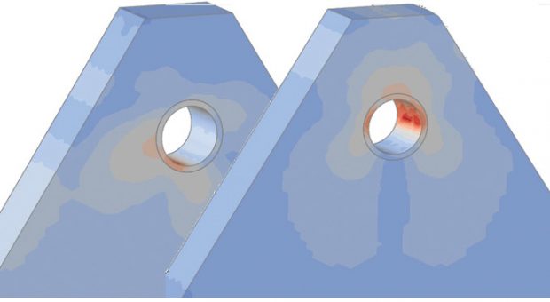
Fig. 9: von Mises stress plot for both load cases.


Latest News
April 1, 2018
This month’s walkthrough looks at solidThinking Inspire 2018 from Altair. This is a structural optimization program designed to provide a complete workflow from geometry creation and or manipulation, through FE analysis to topology optimization and geometry shape fitting of the resultant configuration.
You can view the complete model build in an online video at digitaleng.news/de/inspire.
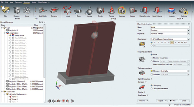 Fig. 1: Screen layout with topology optimization setup in progress.
Fig. 1 shows the Inspire layout, partway through a topology optimization exercise. The main graphics area shows the geometry being reviewed. The very top-level menu controls the major activities such as Geometry (building and manipulating), Structure (setting up FEA and Optimization), View (controlling the User Interface) and File (normal file operations).
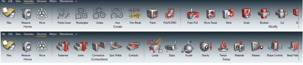 Fig. 2: Toolbars under Geometry menu (top) and Structure menu (below).
Below this is the toolbar ribbon that contains icons to drive the various tasks. The toolbar changes, dependent on the main menu action chosen. Fig. 2 shows the toolbar under the Geometry menu selection (upper) and under the Structure menu selection (lower).
A small toolbar is positioned in the lower left of the screen area to control screen views, orientation, entity visibility etc. A unit selector is positioned in the lower right area of the screen.
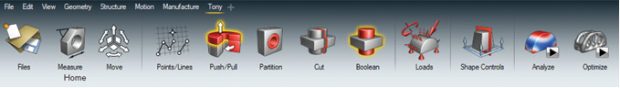 Fig. 3: Custom toolbar.
A feature that may be useful for first-time users is the ability to create a custom toolbar, composed of icons drawn from any of the menu areas. In Fig. 3 I have created a simplified workflow (called Tony) that allows some geometry manipulation, basic loads and boundary condition setup and the ability to analyze and optimize.
The home icons are always present. Separators can be inserted to further clarify the icon context in the workflow, and icons can be dragged left and right. Here, I have split up geometry, loads and boundary conditions, shape controls, and analysis/optimize as distinct stages.
As you explore outside this initial range of features, the corresponding icons can be added to your custom toolbar. This provides a comfortable platform for self-training—or instructor-led training as I show in the accompanying video.
Minimalist Approach
The Inspire house-style is minimalist. Only a relatively small number of icons are present, but their versatility allows a wide range of functionality to be supported. This versatility is shown in the number of options associated with each.
Fig. 4 shows the “Loads” icon. The title is a bit of a misnomer as the icon supports all of the actions shown in the exploded labeling that I have added.
Hovering over each region highlights the required action. This was a bit bewildering at first, and I recommend exploring and practicing with each icon until you are comfortable with its usage. Once each icon is understood, the workflow is visual and very efficient. Notice that Inspire uses the term “support” instead of the usual “constraint”—presumably to avoid confusion with optimization constraints. The little object I have highlighted looks like a suitcase. It is a nice visual clue that unpacks to allow allocation of loads and boundary conditions across a range of load cases. This underpins how important multiple loading conditions are for practical optimization studies.
The Optimization Task
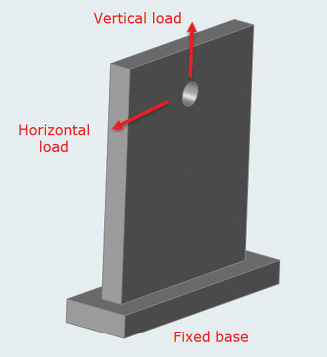 Fig. 5: Initial design space, loading and constraint.
My objective was to create a lug-like configuration starting from the geometry shown in Fig. 5. The vertical part is the design space; the base is a non-design space.
The lug will carry axial loads and side loads. From engineering basics, a lot of the material is not needed above the hole. A tighter initial design space can be defined and has the advantage of reducing the element count in the underlying FEA and making the target Volume Fraction reduction more focused on critical material.
A 50% Volume Fraction used on 20 cubic inches, with 10 cubic inches is redundant and is not effective in driving toward a useful configuration. If the redundancy is removed, then 50% Volume Fraction is literally attacking the meat of the problem in the 10 cubic inches of design space left. Conversely, if too much material is clipped from the initial design space, then the final configuration can be skewed away from a more “natural” result. In this lug, the width is a controlling factor. The bending load case would naturally want a wide base to provide the biggest reacting couple. So, my width limit skews the resulting configuration.
It is a good idea to make this kind of assessment of design space, maybe even to try a set of exploratory FEA studies on broad design space options to understand useful limits.
The Model Setup
I want to slice the corners off of my initial design space to make the topology search more efficient as described. Inspire has some neat tools to do this within a versatile geometry creation and manipulation set. By clicking on the line feature in the Points/Lines icon, a sketching toolbar appears. Two lines are snapped to the corners of the surface. The new faces created by the line intersections are then pulled through the body using the Push/Pull icon, creating an extruded cut.
I am loading the inside of the hole, so the material immediately abutting the load must remain intact by designating it a non-design space. The Partition Icon is used to achieve this. An annular ring is partitioned as a separate body by offsetting the hole surface. The thickness of the ring is important. Too thin and the element size will be prohibitively small, too large and the non-design region will dominate the topology configurations.
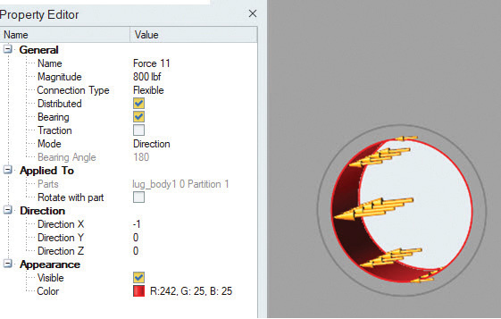 Fig. 6: Load screen picking and Property Editor window.
Now I add the loading. Inspire supports a bearing distribution, which is important for realistic loading. I found the load setup quite tricky, and the best routine for me was to select the force action, select the correct surface area and direction and then convert to a bearing distribution. The Property Editor dialog box can also be opened from the View menu. This means that you can screen pick and correct with a conventional dialog box as shown in Fig. 6. I must admit, however, that millennials may be far more at home with direct icon action than me.
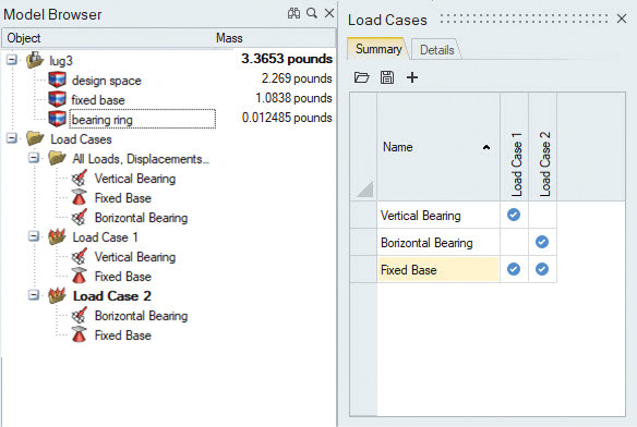 Fig. 7: Load case setup and mass summary.
I created two bearing forces: one laterally and vertically. The non-design partitioned region can also be seen in Fig. 7.
The support (structural constraint) is straightforward in this case, as the complete base is fixed. I created a second load case and then allocated the forces and constraint to each as shown in Fig. 8.
The model setup is shown by using the Model Browser, called from the top menu. I have renamed the forces and support for clarity. Fig. 7 also shows the mass breakdown by part —I have renamed these to clearly identify the mass totals. There is 2.269 lbs. weight available in the design space out of 3.365 lbs. total. The fixed base and bearing ring parts are set as non-design space.
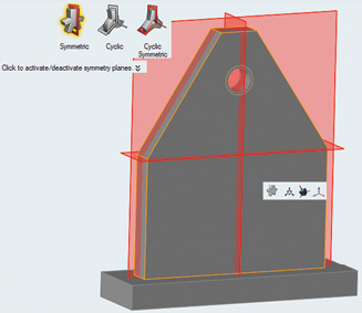 Fig. 8: Symmetry controls.
The final step prior to analysis and optimization is to set the shape controls. I required the design to be symmetric about the vertical centerline to cater for reversed lateral loading. I also wanted a design that was symmetric through thickness. I used planar symmetry, but cyclic; cyclic symmetric can also be used. Control of draw direction is also available, which includes single draw, split draw and overhang. These are critical controls when attempting to generate manufacturable topology configurations.
Fig. 8 shows the symmetry control in action.
The available symmetry planes are shown and can be set relative to any part or to the basic coordinate system. The plane also can be manually shifted. The symmetry plane (or any shape control) can be switched on and off during successive optimization runs to see its influence.
 Fig. 9: von Mises stress plot for both load cases.
Before running the optimization, it is worth doing a check FE analysis to make sure the loads and boundary conditions are set up properly. Fig. 9 shows the results from the two load cases run separately.
The stress values and distributions make sense—which is important as the topology optimization is totally dependent an accurate analysis setup. One trick here is to set the lower stress value on the legend scale to be about -1 times the maximum stress value. This will ensure the contours are clustered more tightly around the maximum value and the stress distribution can be seen more clearly.
The Optimization
Finally, it’s time to go and optimize! I set the optimization Type to Topology. Other options are Topography, Gauge and Lattice. Lattice is one of the new features in 2018. The optimization objective is to maximize stiffness, in other words, to find an efficient design. The target design space volume (Volume Fraction) is 30%. The direct input option below the fixed radio button percentages allows for custom percentages, and also, by stringing values together, a batch of runs. I found this useful once I had explored some of the configurations produced by various Volume Fractions. I could then quickly sweep through a full range. There is no constraint on stress or specific deflection values.
I also did a parallel study that used the minimize mass option as an objective with stress as a constraint. Stress is expressed as a Factor of Safety and is a global measure.
The minimum feature thickness is set at 0.25 in. There are two considerations here; from a design point of view, there will be a minimum practical feature size. If this is set very small, then we allow “filigree” strands of material. This could be a goal—to seek a more organic type of shape. If this is set very large, then the structure becomes chunky and the volume fraction target may not be achievable. The most efficient designs have more distributed material.
The other consideration is the number of elements. If we demand a very small minimum feature size, then the mesh must be able to represent the resultant configuration—which could mean a large number of elements.
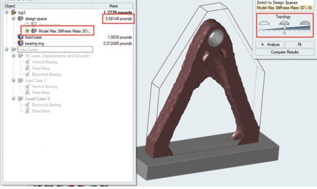 Fig. 10: Topology at 30% Volume Fraction.
Fig. 10 shows the topology optimization result.
The brown object is a surface fit through the remaining material in the topology optimization mesh. The Model Browser reports the new design space mass, as highlighted in the figure.
Investigating the Results
A slider bar (highlighted in Fig. 10) can be moved to adjust the amount of material displayed. This is essentially juggling with the interpolation of the “solid” material in design space. Inspire uses the SIMP method of topology optimization (see digitaleng.news/de/topology-optimization). This means the relative material density is varying from close to zero (material not present) to 1.0 (material present). The “gray” area in between is very much subject to interpretation, particularly in a coarse mesh.
The central position is the baseline topology optimization result. If the configuration changes a lot with a small slider bar movement, then the configuration is not very representative of a “real” structural configuration. The mesh may be too coarse, or the Volume Fraction may just not be feasible with design space and loading provided. The configuration is a very rough suggestion at that point. Bear in mind that aggressive Volume Fraction targets will often produce disconnected configurations. The slider bar also can be used to see if disconnected regions will join up, with a small increase in mass. The changing mass is updated in the Model Browser window. If, however, there is little change in the configuration as the slider bar is moved, then the candidate configuration is much more promising.
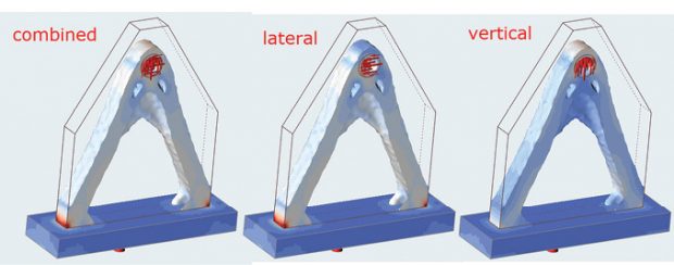 Fig. 11: FE Analysis of the optimized configuration.
Under the slider bar is an Analyze button. This carries out an FE analysis on the configuration and interpolates the stress distribution Fig. 11 shows the result of the analysis, with the two load cases shown.
The combined stress plot is an envelope of the highest stresses seen in the load cases. In this case the lateral (i.e., bending) case dominates. For complex loading scenarios, it is useful to see the design drivers among the load cases.
The next button available is Fit; this fits a set of smoothed surfaces to the optimized configuration. If the surfaces are continuous, then a “smooth” label is appended to a new part name generated. This can be exported as a set of surfaces, as opposed to an STL format. This should help in further geometry manipulation required to turn the configuration into a manufacturable part.
Finally, the Compare button allows the comparison of metrics across a set of optimization runs. Fig. 12 shows the resulting spreadsheet format.
In this case I have tabulated the Mass against Compliance for a set of optimization runs. The columns and parameters can be arranged, ordered and filtered to suit your investigation. Double clicking on a row will pop the configuration open in the graphics window. Here, I set the Mass to ascend and show the corresponding Compliances. I have run a large batch of topology configurations. Several of the low mass configurations have very large compliances as they become very spindly. I have clipped them out of the review table so that they don’t distort the trend.
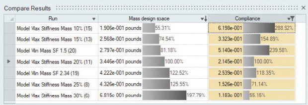 Fig. 12: The Compare spreadsheet.
By clicking in the corner of the spreadsheet all the cells are highlighted and can be copied to the clipboard, and then into Excel. I mentioned I had carried out a parallel study using mass minimization subject to a stress constraint. I was able to export all the data and produce the Excel graph shown in Fig. 13 to see trends.
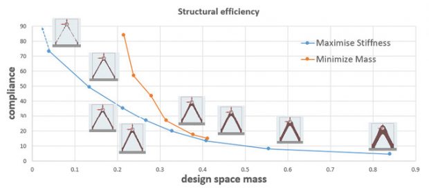 Fig. 13: Two parallel optimization studies.
The first curve shows configurations achieved by maximizing stiffness for a given target Volume Fraction (30% down to 8%). Each point is an efficient structure. Below 0.3 lbs. mass the structures are not realizable due to high stresses, deflections or badly connected structure. The compliance (1/stiffness) shoots up as the configurations get more absurd.
The second curve shows the effect of minimizing mass with a stress constraint. The stress constraint has been relaxed progressively to allow lighter mass configurations.
There is an interesting crossover where the two curves meet at around 0.3 lbs. mass. The configurations are quite similar here, and this could represent an overall efficient solution. The curves do provide useful design information on which to make decisions about what configuration to select to work up into a manufacturable component. Inspire has allowed a rapid investigation across a range of efficient candidate configurations.
More Features to Explore
I mentioned the surface fit option that can export smoothed geometry for design workup. Another very powerful alternative is to use the Inspire PolyNURBS tool. This interactively fits and manipulates surfaces to the topology configuration via a host of methods. It is fun to use and can produce very useful geometry. It deserves its own review, so watch this space.
For More Info
Editor’s Note: This is one of a new series of overview articles looking at simulation and optimization software products. Each review takes the format of a walkthrough using a simple structural example. The full capabilities of each product cannot be covered in a few pages, but we hope to give you a feel for the basic workflow required for each product.
Each overview represents Tony Abbey’s independent assessment and is not sponsored in any way by the companies developing the products. However, in many cases, he is indebted to the companies for supplying temporary licenses to allow the reviews to be carried out.
Tony Abbey teaches both live and e-Learning classes for NAFEMS. He also provides FEA consulting and mentoring. Contact [email protected] for details.
Subscribe to our FREE magazine, FREE email newsletters or both!
Latest News
About the Author
Tony Abbey is a consultant analyst with his own company, FETraining. He also works as training manager for NAFEMS, responsible for developing and implementing training classes, including e-learning classes. Send e-mail about this article to [email protected].
Follow DE

